8. Batch Slurry Adsorption#
In this notes we will use an example problem to introduce material balances in slurry adsorption processes. We will consider a Batch, process configuration and then its extension to a continuous process configuration.
8.1 Problem Statement#
A water purification process is carried out via batch adsorption. The initial concentration of the pollutant is 0.1 \([mol l^{-1}]\), and it needs to be lowered by at least an order of magnitude. The process is carried out in batches characterised by a water volume \(V_{\ell}\) of 2 \(m^3\), in which \(100\,kg\) of adsorbent are dispersed to form a slurry. The adsorbent is characterised spherical particles with an average radius of 1 \(mm\) and density of \(700 kg\,m^{-3}\). The pollutant adsorption on the surface of the stationary phase particles is well described by a linear isotherm \(q=Hc^*\) with \(H=1\times{10^{-1}} [dm]\). The liquid-side mass transfer coefficient is \(k_{\ell}=1\times{10^{-8}}\,[m h^{-1}]\).
Is it possible to carry out the requested purification with the operation parameters described in the problem statment?
If this is the case how much time does it take to lower the pollutant concetration to the target specification?
8.2 Material Balance in a Batch Slurry adsorption process#
Let us begin by writing the material balance for a batch membrane separator.
Since we have a batch system, no inlet or outlet streams are present and we can write:
Where \(V_{\ell}\) is the volume of the liquid phase (it can be considered constant), \(c_0\) is the initial concentration of pollutant in solution, \(c\) is the instantaneous concentration of pollutant in solution, \(q\) the instantaneous surface concentration of pollutant adsorbed on the stationary phase and \(S_p\) the total surface exposed by the stationary phase particles.
Mass transfer in these cases is dominated by bulk transport on the liquid side, thus the flux \(J\) of the pollutant leaving the fluid phase to be incorporated in the stationary phase can be written as:
where \(k_\ell\) is the mass transfer coefficient on the liquid side, and \(c^*\) is the equilibrium concentration, reached at the solid/liquid interface. \(J\) has the units of number of moles per unit time per unit surface.
The differential material balance on the solute concentration can thus be written as:
Where \(a\) represents the particles surface area per unit of fluid volume.
The equilibrium of the adsorption process is well captured by a linear isotherm:
Using Eq. (88) and (91), Eq. (89) can be rewritten as:
Defining: \(\beta=\left(1+\frac{V_\ell}{HS_p}\right)\), and \(\alpha=\frac{V_\ell}{HS_p}\), one gets:
which is a first order, non homogeneous ODE in the form \(y^\prime+C_1y=C_2\) with constant \(C_1\) and \(C_2\) coefficients.
In order to solve our problem Eq. (93) should either numerically or analytically. In this case the analytical solution can be obtained from the general solution for ODEs in the form:
where \(A(t)=\int{C_1dt}\)
In our case:
\(C_1=k_\ell{a\beta}\), thus \(A(t)=k_\ell{a\beta}\,t\)
\(C_2=k_\ell{a\alpha}c_0\),
thus:
putting everything together:
The constant \(C_1\) can be computed from the initial conditions: at \(t=0\) \(c(t)=c_0\), therefore:
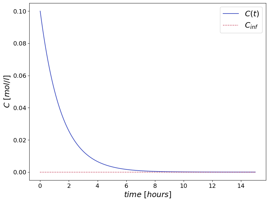
The final solution for the time-dependent concentration profile \(c(t)\) is:
The performance of a batch slurry process in removing the concentration in the fluid phase is limited, i.e. the concentration has an asymptotic behavior in time \(\lim_{t\to\infty} c(t) = \frac{\alpha{c_0}}{\beta}\).
import numpy as np
import matplotlib.pyplot as plt
from matplotlib.pyplot import cm

#Plotting
figure=plt.figure()
axes = figure.add_axes([0.1,0.1,1.2,1.2])
plt.xticks(fontsize=14)
plt.yticks(fontsize=14)
N = 500 #number of points
time = np.linspace(0,15, N)

#particles mass
pm=100; #kg
#particles volume
pV=100/700; #m^3

#single particle volume
radius=1E-3;
uV=(4/3)*np.pi*np.power(radius,3);
uS=4*np.pi**np.power(radius,2);

#number_of particles
NP=pV/uV;
Sp=NP*uS; #particles surface

#Batch volume
Vl=2; #m^3
#Mass transfer
kl=1E-8; #m/h
#Equilibrium
H=1E-1; #

#Analytical solution 1
C0=0.1; #mol/l
alpha=Vl/H/Sp;
beta=1+alpha;
a=Sp/Vl;
C_inf= np.ones(np.size(time)) * C0*alpha/beta
C = C0/beta * (np.exp(-kl*a*beta*time)+alpha)

color=iter(cm.coolwarm(np.linspace(0,1,2)))
c=next(color)
axes.plot(time,C, marker=' ',c=c)
c=next(color)
axes.plot(time,C_inf,marker=' ',linestyle='dotted',c=c)

plt.title('', fontsize=18);
axes.set_xlabel('$time\,\,[hours]$', fontsize=18);
axes.set_ylabel('$C\,\,[mol / l]$',fontsize=18);
axes.legend(['$C(t)$','$C_{inf}$'], fontsize=18);
8.3 Continuous Slurry Adsorption#
The slurry adsorption process can be carried out in a continuous mode. In this mode both the adsorbent and the fluid phase are continuously fed into and removed from a stirred tank.
In a continuous process it is convenient to define \(a\) as:
where \(Q\) is the volumetric flowrate of the liquid phase, ans \(S\) is the mass flowrate of the solid adsorpbent phase, and \(\sigma\) is the surface area per unit mass of the adsorbent.
In this context the differential material balance on the solute concentration used to solve the unsteady state batch process should be rewritten as:
where \(\tau\) is the residence time, \(c_{out}\) the concentration in the liquid phase in the unit, \(c_{in}\) the concentration in the feed, and \(a\) the amount of surface of the stationary phase particles per unit volume of the liquid phase.
This expression should solved with the adsorption isotherm \(q=kc^*\), where \(q\) is the amount adsorbed per kg of stationary phase, \(c\) is the molar concentration in solution and \(k\) is the partition coefficient typically expressed in [l kg\(^{-1}\)], and with the global material balance at steady state, which reads:
Contributions#
Romain Dujardin, 2 May 2022
Salar Rahbari Namin, 8 Feb 2021
Nikita Gusev, 9 Feb 2021