Week 10 - Exercise#

Problem Statement#

Consider a drying process evolving through two stages of i constant drying rate, and ii falling rate (first order kinetics).

During stage i the drying rate per unit area is constant, and indicated with \(R_c=m\times{f_c}=const\).

Where:

\(m\) is a drying rate constant
\(f_c=w_c-w_e\)
\(w_c\) is the critical moisture content
\(w_e\) is the equilibrium moisture content
\(w_0\) is the initial moisture content

During stage ii the rate of drying is proportional to the free moisture content (\(f=w-w_e\)). The falling rate regime stops at the rquilibrium moisture content \(w_e\).

Tasks#

Derive an expression for the time necessary to reduce the moisture content from \(w_0\) to \(w_c\).
Derive an expression for the time necessary to reduce the moisture content from \(w_c\) to \(w_e\) in the (linear) falling regime.
Derive an expression for the time necessary to reduce the moisture content from \(w_0\) to \(w_e<w<w_c\).
If a system, characterised by critical moisture content of 18% and an equilibrium moisture content of 2% takes 7300 seconds to reach a final moisture content of 5% from an initial moisture content of 20%, how long will it take, in the same conditions, to dry a system from 30% to 3%.
For the same system produce a plot of the drying time as a function of the kinetic constant m.

Solution#

Task 1.#

In order to derive an expression for the time necessary to obtain a reduction in the moisture content from an initial value \(w_0\) to the critical moisture content \(w_c\) we shall start by realising that for \(w\geq{w_c}\) the rate of drying (per unit area) \(R=const=R_c=m(w_c-w_e)\).

Hence we can write the rate of reduction in moisture content \(\frac{dw}{dt}\) as:

\[ \frac{dw}{dt}=-R_cA \]

which can be solved by separating the variables

\[ -\frac{dw}{R_cA}=dt \]

and integrating:

\[ -\frac{1}{AR_c}\int_{w_0}^{w_c}dw=\int_{0}^{t_c}dt \]

leads to:

\[ t_c=\frac{w_0-w_c}{AR_c}=\frac{w_0-w_c}{mA(w_c-w_e)} \]

Task 2.#

In order to derive an expression for the time necessary to obtain a reduction in the moisture content from the critical value \(w_c\) to the equilibrium moisture content let us begin first by deriving an expression for a generic \(w_e\geq{w}<w_c\). In this case we know that the rate is linearly dependent on \(w\) accordig to the expression given in the text \(R=m(w-w_e)\). The rate of reduction in moisture content \(\frac{dw}{dt}\) now becomes:

\[ \frac{dw}{dt}=-mA(w-w_e) \]

which can be solved again by separating the variables

\[ -\frac{1}{mA}\frac{dw}{w-w_e}=dt \]

and integrating:

\[ -\frac{1}{mA}\int_{w_c}^{w^\prime}\frac{dw}{w-w_e}=\int_0^{t_w}dt \]

leads to:

\[ t_w=\frac{1}{mA}\ln\left(\frac{w_c-w_e}{w-w_e}\right) \]

we note that since \({w-w_e}\) is at the denominator,

\[ \lim_{w\rightarrow{w_e}}\frac{1}{mA}\ln\left(\frac{w_c-w_e}{w-w_e}\right)=+\infty \]

so for the moisture content approaching iuts equilibrium value the time necessary diverges.

Task 3.#

The total time necessary to dry from an initial moiusture content \(w_0>w_c\) to a final moisture content \(w<w_c\) is equal to:

\[ t_{tot}=\frac{1}{mA}\left(\frac{w_0-w_c}{w_c-w_e}+\ln\frac{w_c-w_e}{w-w_e}\right) \]

Task 4.#

Using the expression derived earlier one can compute first

\[ mA=\frac{1}{t_{tot,1}}\left(\frac{w_{0,1}-w_c}{w_c-w_e}+\ln\frac{w_c-w_e}{w_1-w_e}\right) \]

and then once \(mA\) is known,

\[ t_{tot,2}=\frac{1}{mA}\left(\frac{w_{0,2}-w_c}{w_c-w_e}+\ln\frac{w_c-w_e}{w_2-w_e}\right) \]

import numpy as np

w_e=0.02
w_c=0.18

w0_1=0.2
w_1=0.05
t_1=7300


mA=(1/t_1)*((w0_1-w_c)/(w_c-w_e)+np.log((w_c-w_e)/(w_1-w_e)))
            
w0_2 = 0.3
w_2 = 0.03
            
t_2=(1/mA)*((w0_2-w_c)/(w_c-w_e)+np.log((w_c-w_e)/(w_2-w_e)))
            
print("\nThe drying time is", f"{t_2:.4}", "[s]") 

The drying time is 1.429e+04 [s]

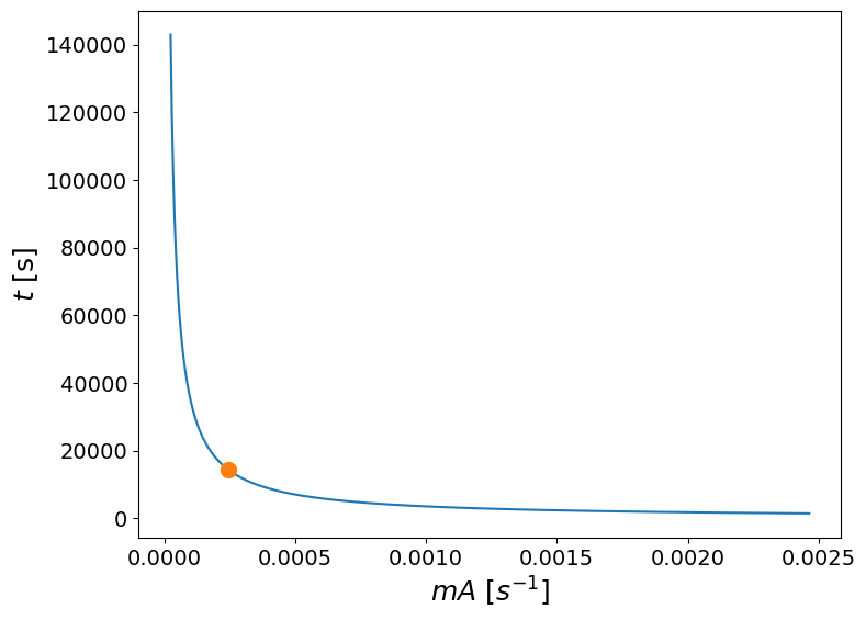
Task 5.#

One cannot plot the dependence of the time on m alone, but the term mA can be used instead.

import numpy as np
import matplotlib.pyplot as plt 
from matplotlib.pyplot import cm

# Data
N=1000
mA_v = np.linspace(mA/10,10*mA, N)
t_v=(1/mA_v)*((w0_2-w_c)/(w_c-w_e)+np.log((w_c-w_e)/(w_2-w_e)))

#Plotting
figure=plt.figure()
axes = figure.add_axes([0.1,0.1,1.2,1.2])
plt.xticks(fontsize=14)
plt.yticks(fontsize=14)
axes.plot(mA_v,t_v, marker=' ') 
axes.plot(mA,t_2,marker='o',markersize=10)
axes.set_xlabel('$mA$ [$s^{-1}$]', fontsize=18);
axes.set_ylabel('$t$ [s]',fontsize=18);

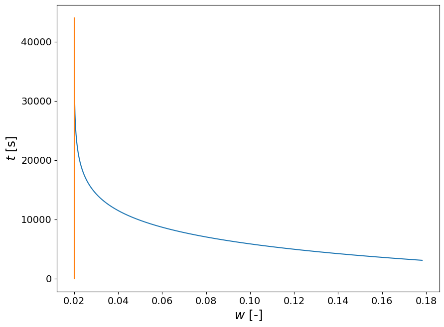
Additional info#

Asymptotic behaviour of the time for the moisture content reaching the equilibrium moisture content:

import numpy as np
import matplotlib.pyplot as plt 
from matplotlib.pyplot import cm

# Data
N=1000
ww = np.linspace(w_e*1.01,w_c*0.99, N)
t_div=(1/mA)*((w0_2-w_c)/(w_c-w_e)+np.log((w_c-w_e)/(ww-w_e)))


#Plotting
figure=plt.figure()
axes = figure.add_axes([0.1,0.1,1.2,1.2])
plt.xticks(fontsize=14)
plt.yticks(fontsize=14)
axes.plot(ww,t_div, marker=' ')
axes.plot(np.array([w_e, w_e]),np.array([0, 44000]))
axes.set_xlabel('$w$ [-]', fontsize=18);
axes.set_ylabel('$t$ [s]',fontsize=18);

Contributions#

Nikita Gusev, 29 March 2021

PSSP Virtual Notebook

Week 10 - Exercise

Contents