4. Membrane Processes Layouts

In this set of notes we will use an example ultrafiltration process to introduce material balances in different process configurations. We will consider a Batch, semi-Batch (feed and bleed) and continuous membrane processes to develop general ideas around material balances in membrane units. Every example will be introduced by a slight variant of a common problem statement.

4.1 Batch

Problem Statement

500 l of fruit juice are concentrated from an initial solid-residue content of 0.05 kg/l to a solid-residue content of 0.2 kg/l through a batch microfiltration process. The total area of the membrane is of 20 \(\mathrm{m^2}\) and the flux of pure water through the membrane is captured by the empirical expression: \(J=BC^{-1} [m/h]\) with \(B=0.1\) where C is the solid residue concentration in kg/l. Compute the process time necessary to reach the target concentration.

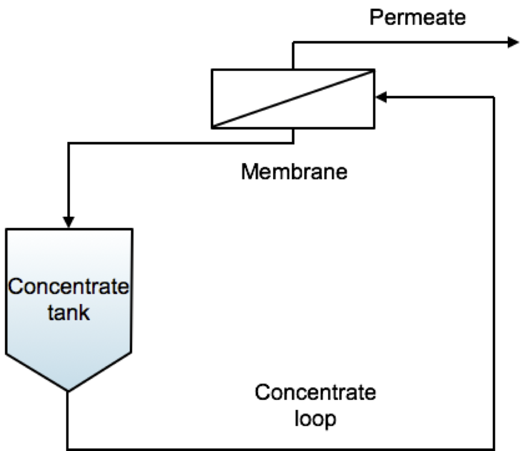
Fig. 1 Schematics of a Batch membrane process.

Solution trace

The global differential material balance (volume basis) reads:

(32)\[ \frac{dV}{dt}=-J\,A \]

where \(V\) is the volume in the concentrate loop, \(J\) the permeate flux per unit area and \(A\) the total membrane area. The permeate flux is defined by the expression:

(33)\[ J=BC^{-1} \]

with \(B=0.1\).

Since the solid residue never leaves the retentate loop, the differential material balance on the solid residue reads:

(34)\[ \frac{dm}{dt}=0 \]

Which means that the total mass of solid residue is constant and equal to its initial mass:

(35)\[ m=m_0=V_0C_0 \]

The global differential material balance can thus be rewritten as:

(36)\[ \frac{dV}{dt}=-J\,A=-\frac{B}{V_0C_0 }AV \]

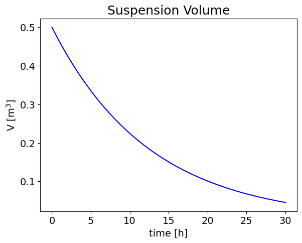
In this simple case it can be integrated analytically to compute the volume as a function of time:

(37)\[ \int_{V_0}^{V^{\prime}}\frac{dV}{V}=\int_0^{t^{\prime}}-\frac{B}{V_0C_0 }Adt \]

(38)\[ \int_{V_0}^{V^{\prime}}\frac{dV}{V}=\left[\ln{V}\right]^{V^{\prime}}_{V_0}=\ln\left(\frac{V^\prime}{V_0}\right) \]

(39)\[ \int_0^{t^{\prime}}-\frac{B}{V_0C_0 }Adt=-\frac{B}{V_0C_0 }At^\prime \]

Putting together both sides of the equation and substituting \(V^\prime\) with \(V\) for the sake of simplicity in the notation we get:

(40)\[ V(t)=V_0e^{-\frac{B}{V_0C_0 }At} \]

which describes the time dependence of the volume in the batch membrane separator.

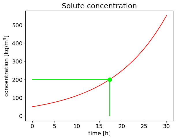
The concentration can thus be calculated as:

(41)\[ C(t)=\frac{m}{V(t)}=\frac{C_0V_0}{V_0}e^{\frac{B}{V_0C_0 }At}={C_0}e^{\frac{B}{V_0C_0 }At} \]

The process time necessary to obtain a solid residue concentration of 0.2 \([kg/l]\) is of 17.3 \([h]\)

Numerical solution

import numpy as np
import matplotlib.pyplot as plt 
from scipy.optimize import fsolve

# Parameters: 
N = 500 #number of points
time = np.linspace(0, 30, N)

#Every length in m

A=20;  #m^2
B=0.1;
C0=0.05*1E3; #kg /l * dm^3/m^3
V0=500*1E-3; #l * m^3/dm^3

C_specific = 0.2*1E3

#Operating Equation
C = C0*np.exp(B*A/V0/C0*time) 
V = V0*np.exp(-B*A/V0/C0*time) 

def equation(proc_time):
    eq1 = C0*np.exp(B*A/V0/C0*proc_time) - C_specific
    return eq1

process_time = fsolve(equation,1)

#Plotting
figure=plt.figure()
axes = figure.add_axes([0.1,0.1,0.8,0.8])
plt.xticks(fontsize=14)
plt.yticks(fontsize=14)
axes.plot(time,V, marker=' ' , color='b')

plt.title('Suspension Volume', fontsize=18);
axes.set_xlabel('time [h]', fontsize=14);
axes.set_ylabel('V [m$^3$]',fontsize=14);

figure=plt.figure()
axes = figure.add_axes([0.1,0.1,0.8,0.8])
plt.xticks(fontsize=14)
plt.yticks(fontsize=14)
axes.plot(time,C, marker=' ' , color='r')
axes.plot(np.array([process_time[0],process_time[0]]),np.array([0, C_specific]), marker=' ' , color='lime', markersize=3)
axes.plot(np.array([0,process_time[0]]),np.array([C_specific, C_specific]), marker=' ' , color='lime', markersize=3)


axes.plot([process_time,process_time],[0, C_specific], marker=' ' , color='lime', markersize=3)


axes.plot(process_time,C_specific, marker='o' , color='lime', markersize=10)

plt.title('Solute concentration', fontsize=18);
axes.set_xlabel('time [h]', fontsize=14);
axes.set_ylabel('concentration [kg/m$^3$]',fontsize=14);

print("The process time necessary to obtain a solid residue concentration of", C_specific, "[kg/l] is:", process_time, "[h]") 

The process time necessary to obtain a solid residue concentration of 200.0 [kg/l] is: [17.32867951] [h]

4.2 Feed and Bleed

Feed and Bleed: Problem Statement

500 l of fruit juice are concentrated in 5 h of steady state operation from an initial solid-residue content of 0.05 \(kg/l\) through a feed and bleed process. The total area of the membrane is of 20 \(m^2\) and the flux of pure water through the membrane is captured by the empirical expression: \(J=BC^{-1} [m/h]\) with \(B=0.1\) where C is the solid residue concentration in kg/l. Is the steady state concentration of the retentate compatible with the specifics of 0.2 \(kg/l\)?

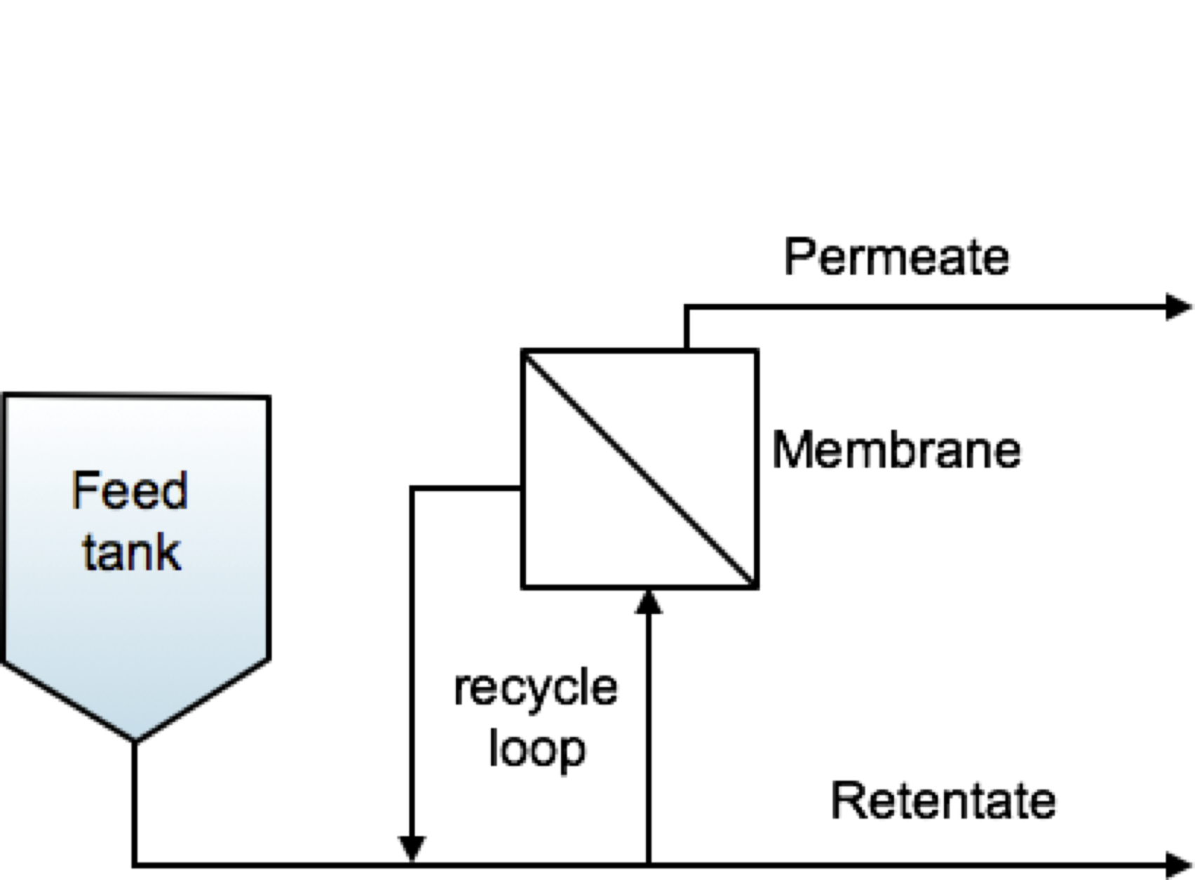
Fig. 2 Feed and Bleed process configuration scheme

Feed and Bleed: Solution trace

Also in this case the global differential material balance and the solid-residue material balance can be written as follows:

(42)\[ \frac{dV}{dt}=Q_{IN}-J\,A-Q_{OUT}=0 \]

(43)\[ \frac{dm}{dt}=Q_{IN}C_{IN}-Q_{OUT}C_{OUT}=0 \]

At steady state \({dV}/{dt}=0\) as well as \({dm}/{dt}=0\). The two ODEs become then two algebraic equations that should be solved together to compute the steady state concentration. From the global material balance we get:

(44)\[ Q_{OUT}=Q_{IN}-J\,A=Q_{IN}-\frac{B}{C_{OUT}}A \]

and then, with some manipulations:

(45)\[ C_{OUT}=C_{IN}+\frac{AB}{Q_{IN}} \]

import numpy as np
import matplotlib.pyplot as plt 
from scipy.optimize import fsolve

# data: 
A=20;  #[m^2]
B=0.1;
C0=0.05*1E3; #kg /l * dm^3/m^3
V0=500*1E-3; #l * m^3/dm^3
process_time=5; # [h]

Cout=C0+A*B*process_time/V0


print("The steady state concentration is", Cout, "[kg/m^3]") 

The steady state concentration is 70.0 [kg/m^3]

4.3 Cascade configuration

Problem Statement

500 l of fruit juice are concentrated in 5 h of steady state operation from an initial solid-residue content of 0.05 kg/l through four membrane separation units characterised by a total membrane area of 20 \(\mathrm{m^2}\) each. The flux of pure water through the membrane is captured by the empirical expression: \(J=BC^{-1} [m/h]\) with \(B=0.1\) where C is the solid residue concentration in kg/l.

Is it more efficient to design a single stage configuration with four units in parallel or a cascade configuration with four units in series?

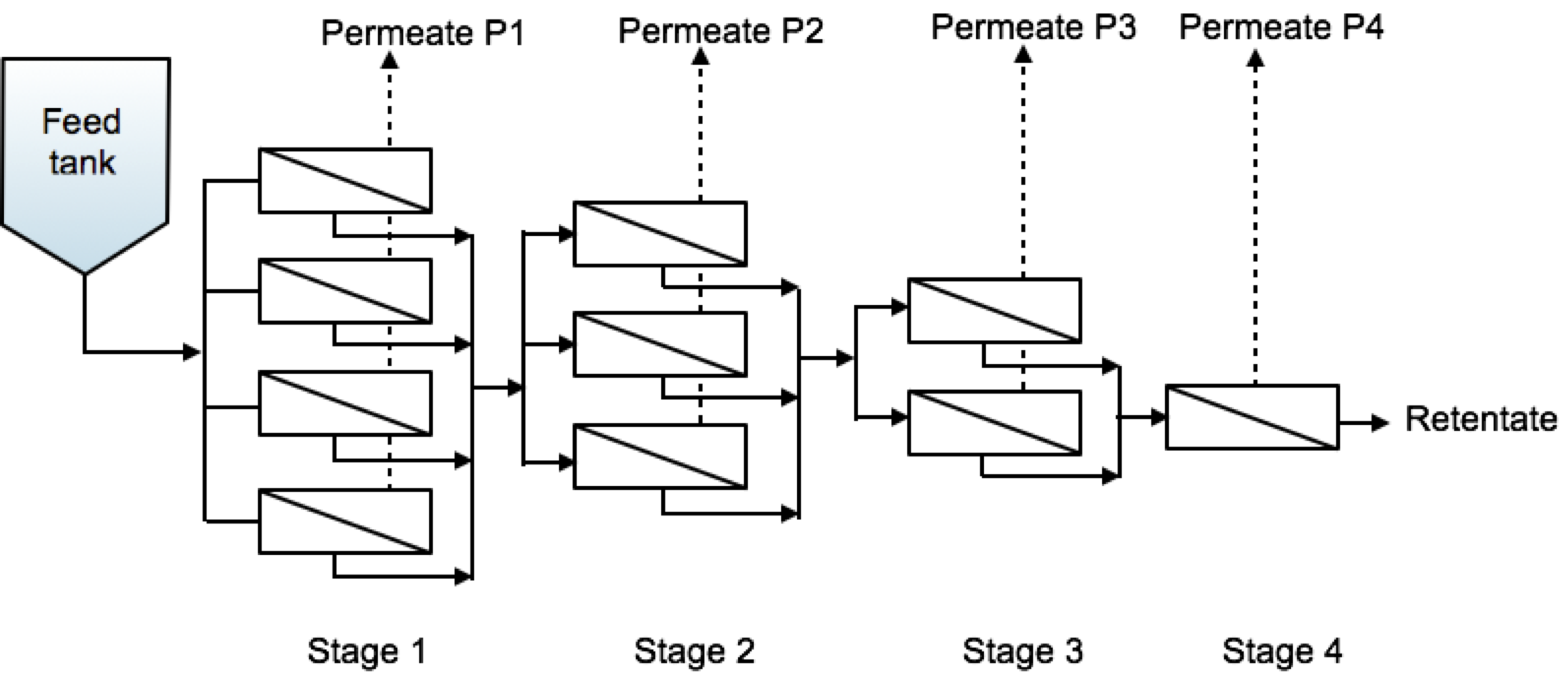
Fig. 3 Cascade configuration schematic representation.

Cascade: Solution trace

Each stage can be treated like a single unit in which the feed stream corresponds to the retentate stream from the previous unit. We can thus define:

(46)\[ C_{OUT,i}=C_{IN,i+1} \]

(47)\[ Q_{OUT,i}=Q_{IN,i+1} \]

where the index \(i\) identifies the stage.

The material balances for each stage at steady state can thus be written as:

(48)\[ \frac{dV}{dt}=Q_{IN,i}-n_iJ(C_{IN,i+1})\,A-Q_{IN,i+1}=0 \]

(49)\[ \frac{dm}{dt}=Q_{IN,i}C_{IN}-Q_{IN,i+1}C_{IN,i+1}=0 \]

where \(n_i\) is the number of modules used in stage \(i\).

For each stage we can thus compute the steady state concentration and concentrate volumetric flow by solving sequentially the following equations:

(50)\[ C_{IN,i+1}=C_{IN,i}+n_i\frac{AB}{Q_{IN,i}} \]

(51)\[ Q_{IN,i+1}=\frac{C_{IN,i}{Q_{IN,i}}}{C_{IN,i+1}} \]

with \(i=1...N\) with \(N\) is the total number of stages.

Numerical Solution

The solution of a cascade composed of any number of stages, each formed by an arbitrary number of modules in parallel can be tackled sequentially through a simple cycle similar to the following, let’s for example consider a system that reflects the sketch above i.e. with 4 stages implementing 4, 3, 2, and 1 modules each:

import numpy as np
import matplotlib.pyplot as plt 
from scipy.optimize import fsolve

# data: 
A=20;  
B=0.1;
C0=0.05*1E3; #kg /l * dm^3/m^3
V0=500*1E-3; #l * m^3/dm^3
process_time=5; # [h]


# The number of elements of this array corresponds to the number of stages. 
# The value in each element is the number of modules per stage. 
n=np.array([4,3,2,1]);

CIN=np.append(C0,np.zeros(np.size(n)-1))
FIN=np.append(V0/process_time, np.zeros(np.size(n)-1));

# Input to the intermediate stages
for i in range(1,np.size(n)): 
    CIN[i]=CIN[i-1]+n[i-1]*A*B/FIN[i-1];
    FIN[i]=CIN[i-1]*FIN[i-1]/CIN[i];

# Output concentration
Cout=CIN[np.size(n)-1]+n[np.size(n)-1]*A*B/FIN[np.size(n)-1];

print("The steady state concentration is", Cout, "[kg/m^3]") 

The steady state concentration is 720.7199999999999 [kg/m^3]

In order to answer the problem request one should solve the system for two different configurations. In the first, representing a single-stage configuration with four membrane units in parallel, the number of stages should be set to \(N=1\) and the number of units in the first stage \(n_1\) to 4.

# The number of elements of this array corresponds to the number of stages. 
# The value in each element is the number of modules per stage. 
n=np.array([4]);

CIN=np.append(C0,np.zeros(np.size(n)-1))
FIN=np.append(V0/process_time, np.zeros(np.size(n)-1));

# Input to the intermediate stages
for i in range(1,np.size(n)): 
    CIN[i]=CIN[i-1]+n[i-1]*A*B/FIN[i-1];
    FIN[i]=CIN[i-1]*FIN[i-1]/CIN[i];

# Output concentration
Cout=CIN[np.size(n)-1]+n[np.size(n)-1]*A*B/FIN[np.size(n)-1];

print("The steady state concentration is", Cout, "[kg/m^3]") 

The steady state concentration is 130.0 [kg/m^3]

In the second the number of stages should be set to \(N=4\), each of the stages being assembled as a single unit (\(n_i=1\) for \(i=[1, 4]\)).

# The number of elements of this array corresponds to the number of stages. 
# The value in each element is the number of modules per stage. 
n=np.array([1, 1, 1, 1]);

CIN=np.append(C0,np.zeros(np.size(n)-1))
FIN=np.append(V0/process_time, np.zeros(np.size(n)-1));

# Input to the intermediate stages
for i in range(1,np.size(n)): 
    CIN[i]=CIN[i-1]+n[i-1]*A*B/FIN[i-1];
    FIN[i]=CIN[i-1]*FIN[i-1]/CIN[i];

# Output concentration
Cout=CIN[np.size(n)-1]+n[np.size(n)-1]*A*B/FIN[np.size(n)-1];

print("The steady state concentration is", Cout, "[kg/m^3]") 

The steady state concentration is 192.07999999999998 [kg/m^3]

The cascade configuration allows for a more efficient process since it allows to obtain a larger concentration with the same number of modules.