3. The Osmotic Pressure#
3.1 Osmosis#
Osmosis is a mass transfer process that takes place spontaneously when two compartments, containing fluid mixtures of different composition are separated by a semipermeable membrane, i.e. a membrane that restricts the transfer of one of the components across compartments.
For the sake of simplicity, let us consider for now an ideal semipermeable membrane that completely restricts the transfer of the solute, while instead allowing the permeation of a solvent.
Let us consider an initial state characterised by two compartments (1 and 2), at the same temperature T and pressure P. Compartment 1 contains a binary mixture of component B (solute) in component A (solvent), e.g. NaCl in water. Compartment 2 instead contains a pure component A (e.g. pure water).
If the membrane is semipermeable and allows for the passage of the solvent alone the process of osmosis will lead to an equilibrium condition in which:
Component A has transferred from compartment 2 to compartment 1.
An pressure difference between compartments is established, where : \(P_1>P_2\).
The pressure difference between compartments at equilibrium is the osmotic pressure \(\pi=P_1-P_2\).
In the next paragraphs we will see what is the thermodynamic origin of the osmotic pressure.
3.2 Equilibrium Conditions#
In order to understand the origin of the osmotic pressure, i.e. pressure difference induced by a composition difference across compartments separated by a semipermeable membrane, we begin by defining the the equilibrium state for the system described in the previous paragraph. To this aim we can rely on the thermodynamic definition of equilibrium for component A (e.g. water), i.e. the only component that can transfer across the membrane. Equilibrium is defined when \(A\) has the same chemical potential in both compartments
The equilibrium condition is conveniently written introducing fugacity. Fugacity and chemical potential are related by the expression \(\mu_i=\mu_0+RT\ln{f_i}\), where \(\mu_0\) is the chemical potential of an arbitrary reference state.
Equilibrium can conditions are thus equivalently formulated as:
In compartment 1 we have a non-ideal mixture of two components. The fugacity of component A in compartment 1 is thus written as:
where:
\(\gamma_A(T,P_1,x_A)\) is the activity coefficient of specie A in the mixture
\(x_A\) is the molar fraction of component A
\(f_A(T,P_1)\) is the fugacity of the pure component A at temperature \(T\) and pressure \(P_1\)
In compartment 2 we have instewad a pure component A liquid, at temperature \(T\) and pressure \(P_2\). The fugacity of component A in compartment 2 thus simply corresponds to the fugacity of the pure component A at \(T\), \(P_2\):
The Poynting correction In order to define a common reference state between the two compartments we rewrite fugacity of the pure component A at pressure \(P_2\) (\(f_A(T,P_2)\)) as a function of the fugacity of the pure component A at pressure \(P_1\) and of the pressure difference \((P_2-P_1)\).
To do that we express the difference in chemical potential \(\Delta\mu_{P_1\rightarrow{P_2}}\) between pure liquid A at temperature \(T\) and pressure \(P_1\) and pure liquid A at temperature \(T\) and pressure \(P_2\):
where:
the expression introduced for the definition of the \(\Delta\mu\) is the Gibbs Duhem equation (\(d{\mu}=-sdT+vdP\))
\(v\) is the molar volume of the system
Using the definition of fugacity introduced earlier one can thus write:
The fugacity of a pure A liquid at pressure \(P_2\) can thus be written as:
where the term \(\left[\exp\left(\frac{v(P_2-P_1)}{RT}\right)\right]\) is the Poynting correction.
3.3 The Osmotic Pressure#
Given the definition of equilibrium conditions, the expressions of the fugacity of component A in the two compartments 1 and 2, and the Poynting correction given in the previous paragraph we can write:
where \(f_A(T,P_1)\) is the fugacity of the pure component A at pressure \(P_1\), now appearing on both sides of the equation.
We can thus divide both sides by \(f_A(T,P_1)\) to obtain the expression:
Rearranging this expression one obtains:
Recalling that the Osmotic pressure \(\pi=P_1-P_2\) we get:
This expression relates the composition of compartment 1, containing a mixture of components A and B (e.g NaCl in water), to the osmotic pressure generated at equilibrium conditions when such compartment is in contact with a semipermeable membrane that has on the opposite side a compartment filled by pure component A liquid.
Please note that in this expression \(x_A\) is the molar fraction of the solvent (e.g. water). Since we are considering a binary system and from an engineering standpoint what is typically measured is the solute concentration we can rewrite the expression as follows:
Where now \(x_B\) is the molar fraction of component \(B\) (e.g. NaCl). When the solution in compartment 1 is diluted (\(x_B\) small), \(\gamma_A(T,P_1,x_A)\rightarrow{1}\), \(\ln{\left({(1-x_B)}\right)}\rightarrow{-x_B}\) thus:
Where \(c_B\simeq{x_B}v^{-1}\) is the molar concentration of component B, the solute.
3.3.1 Dependence of the Osmotic pressure on the composition of the system#
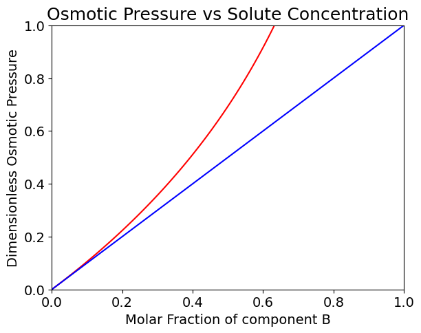
Note that the expression \(\pi={RTc_B}\) is only valid for small molar fractions of component B, the solute.
import numpy as np
import matplotlib.pyplot as plt

# Parameters:
# molar fraction in the feed
N = 100 #number of points
x_B = np.linspace(0, 0.999, N)

#Operating Equation
pi = - np.log(1-x_B)
pi_simple = x_B

#Plotting
figure=plt.figure()
axes = figure.add_axes([0.1,0.1,0.8,0.8])
plt.xticks(fontsize=14)
plt.yticks(fontsize=14)
axes.plot(x_B,pi, marker=' ' , color='r')
axes.plot(x_B,pi_simple, marker=' ' , color='b')
axes.set_xlim([0,1]);
axes.set_ylim([0,1]);
plt.title('Osmotic Pressure vs Solute Concentration', fontsize=18);
axes.set_xlabel('Molar Fraction of component B', fontsize=14);
axes.set_ylabel('Dimensionless Osmotic Pressure',fontsize=14);

Note that the dimensionless osmotic pressure plotted abotve is obtained as \(\pi{v}/RT\).
3.4 Flux of the solvent during Osmosis#
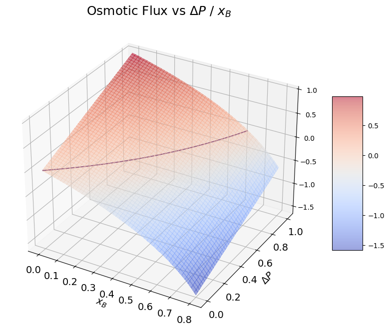
In osmosis the flux of the solvent (component A) through a membrane is driven by the difference between the \(\Delta{P}=P_1-P_2\) across compartments and the osmotic pressure \(\pi\):
where \(p_A\) is the permeability of the membrane with respect to component A.
At equilibrium, when \(\Delta{P}=\pi\) the net flux across compartments is null. Without adding any external pressure the spontaneous direction of the flux is from compartment 2 to compartment 1 (\(J<0\)).
If we add a pressure, such that \(\Delta{P}>\pi\) we induce the opposite flux, from compartment 1 to compartment 2. This process is named reverse osmosis.
import numpy as np
import pandas as pd
from matplotlib import cm
import matplotlib.pyplot as plt
from mpl_toolkits.mplot3d import Axes3D

# Parameters:
# molar fraction in the feed
N = 100 #number of points
DeltaP = np.linspace(0, 1, N)
x_B = np.linspace(0, 0.8, N)
P_A= 1
DeltaP, x_B = np.meshgrid(DeltaP, x_B)

pi = - np.log(1-x_B)

#Flux Equation
J_A = P_A * (DeltaP - pi)


#Plotting

figure=plt.figure(figsize=(10, 8))
#axes = figure.add_axes([0.1,0.1,0.1,1.2,1.2,1.2])
axes = figure.add_subplot(projection='3d')


plt.xticks(fontsize=14)
plt.yticks(fontsize=14)

surf=axes.plot_surface(x_B,DeltaP,J_A,cmap=cm.coolwarm,
                       linewidth=0, antialiased=False,alpha=0.5)

contour=axes.contour(x_B,DeltaP,J_A,[0])

plt.title('Osmotic Flux vs $\Delta{P}$ / $x_B$', fontsize=18);
axes.set_xlabel('$x_B$', fontsize=14);
axes.set_ylabel('$\Delta{P}$',fontsize=14);
figure.colorbar(surf, shrink=0.5, aspect=5);

