1. Material Balances in a Gas Permeation Unit

1.1 Operating Equation

Consider a binary gas phase mixture fed into a perfectly mixed membrane separation unit with molar flow rate \(F_{in}\), and composition \(\vec{z}\). The retentate stream is characterised by molar flow rate \(F_{r}\), and composition \(\vec{x}\), while permeate is characterised by molar flow rate \(F_{p}\) and composition \(\vec{y}\).

Since we are dealing with a binary mixture, in all streams the compositions of A and B complement to 1 (e.g. for the permeate stream \(y_B=1-y_A\)). Hence we drop unnecessary subscripts and indicate with \(z\), \(x\), and \(y\) the molar fraction of component A in the mixture.

The global material balance on the unit reads: \(F_{in}=F_p+F_r\)

The material balance for component A reads: \(F_{in}z=F_py+F_rx\)

Combining these two equations:

\[ F_{in}z=F_py+(F_{in}-F_p)x \]

(1)\[ z=\frac{F_p}{F_{in}}y+(1-\frac{F_p}{F_{in}})x \]

the quantity \(\frac{F_p}{F_{in}}\) is commonly defined as cut and indicated as \(\theta\).

Solving Eq.(1) for \(y\) leads to the expression:

(2)\[ y=\frac{\left(\theta-1\right)}{\theta}x+\frac{1}{\theta}z \]

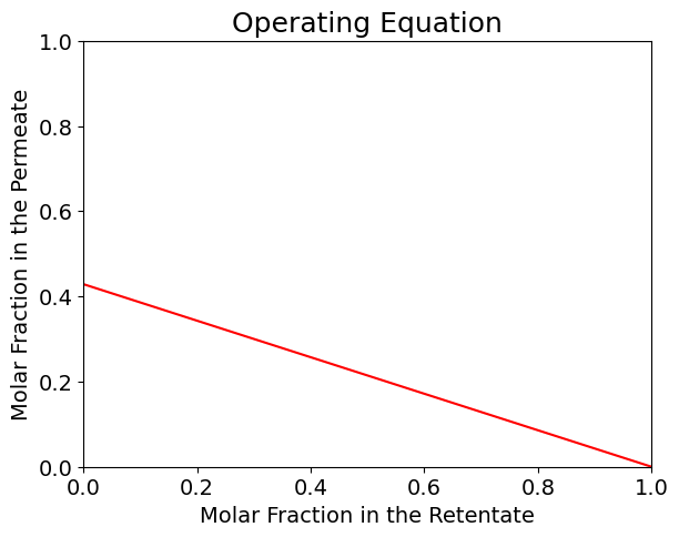
Eq. (2) is typically referred to as the Operating Equation of a perfectly mixed gas phase membrane module.

Graphical Representation

import numpy as np
import matplotlib.pyplot as plt 

# Parameters: 
# cut
theta = 0.7
# molar fraction in the feed
z = 0.3
N = 100 #number of points
x_op = np.linspace(0, 1, N)

#Operating Equation
y_op = ((theta - 1) / theta) * x_op + (z / theta) 

#Plotting
figure=plt.figure()
axes = figure.add_axes([0.1,0.1,0.8,0.8])
plt.xticks(fontsize=14)
plt.yticks(fontsize=14)
axes.plot(x_op,y_op, marker=' ' , color='r')
axes.set_xlim([0,1])
axes.set_ylim([0,1]);
plt.title('Operating Equation', fontsize=18);
axes.set_xlabel('Molar Fraction in the Retentate', fontsize=14);
axes.set_ylabel('Molar Fraction in the Permeate',fontsize=14);

1.2 Rate Transfer Equation

Let us begin by considering that the permeate flow rate of component A is given by its molar flux through the membrane multiplied by the membrane total area:

(3)\[ F_py=J\rho_AA_M \]

where \(J\) is the volumetric flux across the membrane, \(\rho_A\) is the molar density of component A, and \(A_M\) is the total area of the membrane. Applying the solution/diffusion model to define the volumetric flux Eq. (3) becomes:

(4)\[ F_py=\frac{P_A}{l}\rho_AA_M\left(xp_r-yp_p\right) \]

where \(P_A\) is the permeability of the membrane to component \(A\), \(l\) is the thickness of the membrane, \(p_r\) is the pressure on the retentate side, \(p_p\) is the pressure on the permeate side.

The same expression can be written for component \(B\):

(5)\[ F_p(1-y)=\frac{P_B}{l}\rho_BA_M\left((1-x)p_r-(1-y)p_p\right) \]

Both Eq. (4) and (5) can be solved for \(F_p\) and equated, leading to:

(6)\[ \frac{P_A}{y}\rho_A\left(xp_r-yp_p\right)=\frac{P_B}{(1-y)}\rho_B\left((1-x)p_r-(1-y)p_p\right) \]

Eq. (6) can be solved either for \(y\) or for \(x\), the latter being simpler. After some algebraic manipulation the solution for \(x\) is:

(7)\[ x=\frac{y\left[1+\frac{p_p}{p_r}(1-y)\left(\alpha_{AB}\frac{\rho_A}{\rho_B}-1\right)\right]}{\alpha_{AB}\frac{\rho_A}{\rho_B}-\left(\alpha_{AB}\frac{\rho_A}{\rho_B}-1\right)y} \]

where \(\alpha_{A,B}=\frac{P_A}{P_B}\) is the ideal separation factor.

Eq. (7) can be simplified when the gas phase can be considered ideal. In such case \(\rho_A=\rho_B=P/RT\), yielding:

(8)\[ x=\frac{y\left[1+\frac{p_p}{p_r}(1-y)\left(\alpha_{AB}-1\right)\right]}{\alpha_{AB}-\left(\alpha_{AB}-1\right)y} \]

Eq. (8) is called rate transfer equation and together with th operating equation identify the membrane operating conditions in composition space.

Graphical Representation

# Parameters: 
# Ratio between the permeate and retentate side pressures
Pp_Pr = 0.3
# ideal separation factor
alpha = 100
N = 100 #number of points
y_rt = np.linspace(0, 1, N)

#Rate Transfer
x_rt = y_rt * (1 + Pp_Pr * (1-y_rt) * (alpha - 1)) / (alpha - (alpha - 1) * y_rt)

#Plotting
figure=plt.figure()
axes = figure.add_axes([0.1,0.1,1.0,1.0])
plt.xticks(fontsize=14)
plt.yticks(fontsize=14)
axes.plot(x_op,y_op, marker=' ' , color='r')
axes.plot(x_rt,y_rt, marker=' ' , color='b')
axes.set_xlim([0,1])
axes.set_ylim([0,1])
plt.title('Operating and Rate Transfer Equations', fontsize=18);
axes.set_xlabel('Molar Fraction in the Retentate', fontsize=14);
axes.set_ylabel('Molar Fraction in the Permeate',fontsize=14);

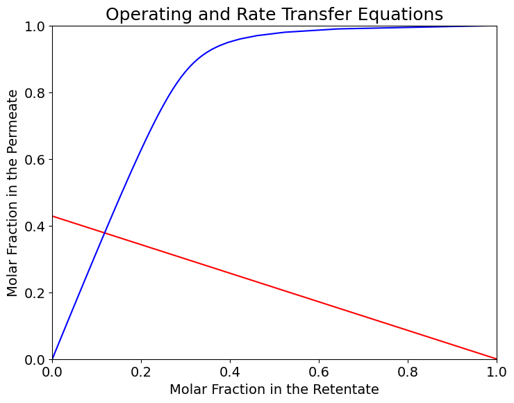
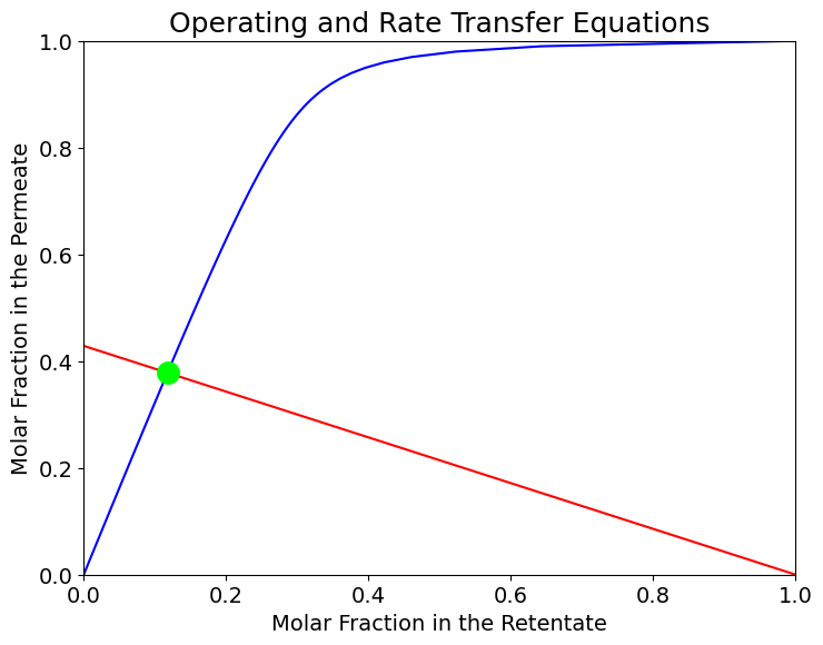
The operating conditions correspond to the interasection of the RT and OP equations, i.e. the solution of a system of equations defined by the operating and rate transfer equations.

Numerical Solution

from scipy.optimize import fsolve

def equations(vars):
    x, y = vars
    eq1 = ((theta - 1) / theta) * x + (z / theta) - y
    eq2 = y * (1 + Pp_Pr * (1-y) * (alpha - 1)) / (alpha - (alpha - 1) * y) - x
    return [eq1, eq2]

x_set, y_set =  fsolve(equations, (1, 1))


#Plotting
figure=plt.figure()
axes = figure.add_axes([0.1,0.1,1.0,1.0])
plt.xticks(fontsize=14)
plt.yticks(fontsize=14)
axes.plot(x_op,y_op, marker=' ' , color='r')
axes.plot(x_rt,y_rt, marker=' ' , color='b')
axes.plot(x_set,y_set, marker='o' , color='lime', markersize=14)
axes.set_xlim([0,1])
axes.set_ylim([0,1])
plt.title('Operating and Rate Transfer Equations', fontsize=18);
axes.set_xlabel('Molar Fraction in the Retentate', fontsize=14);
axes.set_ylabel('Molar Fraction in the Permeate',fontsize=14);


print("Operating point -> x = ", x_set, " y = ", y_set) 

Operating point -> x =  0.11767288696786887  y =  0.3781401912994848

Contributions

• Radoslav Lukanov, 16 Feb 2021

• Garv Mittal, 4 Feb 2024